Abstract

The Monte Carlo method is a numerical approach for solving problems using random sampling. The original motivation for the method was to facilitate the resolution of partial differential equations appearing in natural studies, but has been adopted for the general solution of problems where an analytical solution is not available or too complicated to be used. Typical situations include optimisation, numeric integration, sampling from probability distributions, and random variable computations. This article discusses the fundamental elements of the method and provides guidance for implementation using standard spreadsheet software.

Random variables

A discrete random variable $\xi$ can take values from a discrete set $x_1, x_2, \dots, x_n$ . The discrete random variable is specified by the following table:

$\xi = \left( \begin{array}{cccc} x_1 & x_2 & \dots & x_n \\ \Pr(x_1) & \Pr(x_2) & \dots & \Pr(x_n) \end{array} \right)$

The values $x_1, x_2, \dots, x_n$ can be arbitrary, but the associated probabilities must satisfy two conditions

$0 \leq \Pr(x_i) \leq 1$
$\sum\limits_{i=1}^n \Pr(x_i) = 1$

The expected value $\textbf{E}$ of a discrete random variable is defined as

$\textbf{E}\xi = \sum_ix_i\Pr(x_i)$

The expected value has the following properties, where $c$ is an arbitrary non-random number

$\textbf{E}(\xi + c) = \textbf{E}\xi + c$
$\textbf{E}(c\xi) = c\textbf{E}\xi$

The variance $\textbf{V}$ of a random variable is defined as

$\textbf{V}\xi = \textbf{E}(\xi - \textbf{E}\xi)^2$

The variance has the following properties, where $c$ is an arbitrary non-random number

$\textbf{V}(\xi + c) = \textbf{V}\xi + c$
$\textbf{V}(c\xi) = c^2\textbf{V}\xi$

If a random variable $\xi$ is sampled $N$ times then it will assume values from $x_1, x_2, \dots, x_n$ and the arithmetic mean will be close to $\textbf{E}\xi$

$\frac{1}{N}(\xi1_1 +\xi_2+\dots+\xi_N) \approx \textbf{E}\xi$

The following relationships are valid for independent random variables

$\textbf{E}(\xi\eta)=\textbf{E}\xi\textbf{E}\eta$
$\textbf{V}(\xi+\eta) = \textbf{V}\xi +\textbf{V}\eta$

A continuous random variable is defined over a continuous interval $(a,b)$ with a probability density function (pdf) $p(x)$ . All the properties of discrete random variables also apply to continuous random variables. In addition if $f(x)$ is a continuous arbitrary function then

$\textbf{E}f(\xi) = \displaystyle\int_a^bf(x)p(x)dx$

generally $\textbf{E}f(\xi) \ne f(\textbf{E}\xi)$

Two useful random variables

The random variable $\gamma$ defined over the interval $(0,1)$ with a pdf $f(x) = 1$ is said to be uniformly distributed in $(0,1)$

It can be verified that $\textbf{E}\gamma = \frac{1}{2}$ , and $\textbf{V}\gamma = \frac{1}{12}$ .

The random variable $\zeta$ defined over the interval $(-\infty, \infty)$ with a pdf $p(x) = \displaystyle\frac{1}{\sigma\sqrt{2\pi}}e^{-\displaystyle\frac{(x-a)^2}{2\sigma^2}}$ where $a$ and $\sigma$ are numeric parameters.

It can be verified that $\textbf{E}\zeta = a$ , $\textbf{V}\zeta = \sigma^2$ , and $\Pr(a-3\sigma < \zeta < a+3\sigma) = \displaystyle\int_{a-3\sigma}^{a+3\sigma}p(x)dx = 0.997$

The Central Limit Theorem

A set of $N$ identical independent random variables $\xi_1, \xi_2, \dots \xi_N$ will have identical expected values and variances

$\textbf{E}\xi_1 = \textbf{E}\xi_2 = \dots = \textbf{E}\xi_N = m,\\\textbf{V}\xi_1 = \textbf{V}\xi_2 = \dots = \textbf{V}\xi_N = b^2$

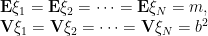
Lets call the sum of these values $\rho$

$\rho = \xi_1 + \xi_2 + \dots + \xi_N$

It can be seen that

$\textbf{E}\rho = \textbf{E}(\xi_1+\xi_2+\dots+\xi_N) = Nm\\\textbf{V}\rho = \textbf{V}(\xi_1+\xi_2+\dots+\xi_N) = Nb^2$

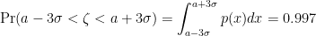
Lets consider now a normal random variable $\zeta$ with the same parameters: $a = Nm, \sigma^2 = Nb^2$

The central limit theorem states that for any interval $(a',b')$ and for a large $N$ the sum of identical random variables is approximate normal

$\Pr(a'<\rho<b') \approx\displaystyle\int_{a'}^{b'}p_\zeta(x)dx$

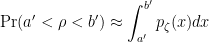
The central limit theorem is also valid for any sum of random variables (not necessarily identical and independent) provided that no single variable plays a significant role in the sum.

The Monte Carlo method

To determine some unknown value $m$ we shall try to find a random variable $\xi$ such that $\textbf{E}\xi = m$ with $\textbf{V}\xi = b^2$ .

Lets consider $N$ independent random variables $\xi_1, \xi_2 \dots \xi_N$ with pdfs identical to $\xi$ . If $N$ is sufficiently large then the pdf of the sum of the random variables $\rho$ will be approximately normal with parameters $a=Nm$ and $\sigma^2 = Nb^2$

$\Pr(Nm - 3b\sqrt{N} < \rho < Nm + 3b\sqrt{N}) \approx 0.997$

Rearranging this equation we arrive at the Monte Carlo formula

$\Pr \left[ \left| \displaystyle\frac{1}{N} \sum\limits_{i=1}^N \xi_i - m \right| < \displaystyle\frac{3b}{\sqrt{N}}\right] \approx 0.997$

From this expression we can determine the expected value of the random variable $\xi$ with an estimation error $\epsilon$ as a function of the number of trials $N$

$\epsilon = \displaystyle\frac{3 b}{\sqrt{N}}$

The method consists of sampling $N$ values of the random variable $\xi$ (determining a single value of each of the variables $\xi_i$ is equivalent to determining $N$ values of a single variable $\xi$ because all these random variables are identical). The arithmetic mean of these values will be approximately equal to $m$ with an error not exceeding $\epsilon$ .

Practical implementation

There are a number of commercial packages that run Monte Carlo simulation, however a basic spreadsheet program can be used in most situations. The generation of multiple trials is implemented by propagating a basic formula $N$ times.

A typical problem consists in the determination of an unknown value $m$ which is the value of a combination of random variables.

Lets assume that the total cost of a project is the sum of the cost of a number of independent activities $A_1, A_2 \dots A_n$ . The cost of each activities $A_i,$ is a random variable which can have a value in the range $(C_i ,C_i+\Delta_i)$ . The total cost is a random variable within the interval $(\min(C_i),max(C_i+\Delta_i))$ . Each of these activities may have a particular probability distribution, and the sum of all these variables will have a composite probability distribution, but thanks to the central limit theorem we can use a uniform distribution without compromising the result.

An important assumption is that each of the variables is independent of the others. This means that the cost of any activity is not influenced by the cost of any other activity.

The general scheme of the Monte Carlo method is as follows:

Generate random values for each of the activity costs
Add these variables in a total project cost
Repeat this operation $N$ times
The expected project cost is the average of the total project cost

The first step is to generate random values for each of the activity costs. Assuming a uniform distribution, we can use the RAND() function to generate random numbers in the interval (0,1) and multiply these by the range of each variable. The range is the difference between the maximum value and the minimum value $(C_i, C_i+\Delta_i)$ .

The cost for Activity $A_i$ will look like this:

$=RAND()*(\Delta_i)+C_i$

To determine the number of iterations we estimate the standard deviation $b$ of the random variable and specify the desired error $\epsilon$ .

We can estimate an upper bound of $b$ by calculating the standard deviation between the maximum, the minimum and average values of the random variable:

$b = STDEV.P(\min(C_i),\max(C_i+\Delta_i),AVERAGE(\min(C_i),\max(C_i+\Delta_i))$

Note that we used the function STDEV.P, which calculates the standard deviation of the entire population, in this case only 3 values.

To calculate $\epsilon$ we set the error $e$ as fraction of the average value of the random variable, calculated between the minimum and the maximum.

$\epsilon = e*\sum\limits_{i=1}^n\displaystyle\frac{2C_i + \Delta_i}{n}$

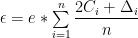
The number of iterations to obtain a result with an error of less than $\epsilon$ is:

$N = \left(\displaystyle\frac{3*b}{\epsilon}\right)^2$

The kurtosis and skewness of the generated distribution will be close to the normal distribution.

Conditional variables

An important assumption is that the random variables are independent. Covariance is defined as:

$\sigma(\xi,\eta) = \textbf{E}[(\xi-\textbf{E}\xi)(\eta - \textbf{E}\eta)]$

If $\xi$ and $\eta$ are independent then $\sigma(\xi,\eta) = 0$ . It should be noted that the converse is not necessarily true; if the covariance of two random variables is zero they are not necessarily independent.

If the simulation model requires conditional random variables then they can be generated using the following algorithm:

Generate two uniform random variables $\gamma_1$ and $\gamma_2$
Generate a third random variable $\gamma_3 = \rho \gamma_1+\gamma_2\sqrt{1-\rho^2}$

Where $\rho_{\xi\eta} = \displaystyle\frac{\sigma(\xi,\eta)}{\sigma_\xi \sigma_\eta}$ is the coefficient of correlation.

Variance Reduction Techniques

The Monte Carlo method produces a result that is the expected value $\textbf{E} \xi$ of the unknown variable $m$ . The confidence interval of this estimator is determined by the variance of the result $\textbf{V} = b^2$ . We shall discuss some techniques to reduce the variance of the Monte Carlo result and hence the confidence interval of the estimate.

Common Random Numbers. If we are comparing two different systems it is better to use the same set of random numbers for both simulation runs. The idea is based on the following property of the variance:

$\textbf{V}(\xi-\eta) = \textbf{V}\xi + \textbf{V}\eta - 2\sigma(\xi,\eta)$

If $\xi$ and $\eta$ are positively correlated with $\sigma(\xi,\eta) > 0$ then the variance of $\xi-\eta$ will be smaller than if $\xi$ and $\eta$ were independent.

Antithetic Variables. If $\gamma$ is uniformly distributed on $(0,1), 1 -\gamma$ is also uniformly distributed. The two random variables are negatively correlated, $\sigma(\gamma, 1-\gamma) < 0$ . The idea is that if $\xi_1$ and $\xi_2$ are two successive results, then

$\textbf{V}\left(\frac{\xi_1 + \xi_2}{2}\right) = \frac{1}{4}\textbf{V}\xi_1 + \frac{1}{4}\textbf{V}\xi_2 +\frac{1}{2}\sigma(\xi_1, \xi_2)$

Therefore if $\xi_1$ and $\xi_2$ are negatively correlated then the variance of $\textbf{V}\left(\displaystyle\frac{\xi_1 + \xi_2}{2}\right)$ is smaller than if the variables are independent.

References

Metropolis, N; Ulam, S (1949) “The Monte Carlo Method”, Journal of the American Statistical Association, No 247, Vol 44

Rob Jeges

Management Science and Philosophy

Tag Archives: random variable

The Monte Carlo method

Abstract

Random variables

Two useful random variables

The Central Limit Theorem

The Monte Carlo method

Practical implementation

Conditional variables

Variance Reduction Techniques

References