Abstract

The diffusion process describes the adoption of a new product by the market. The process has been described by various authors including Rogers (1972) and Bass (1969). This article reviews the main ideas of the model and presents the derivation of key formulas with a discussion of the results.

Introduction

The adoption of a new product by a market is driven by two factors: innovation and imitation. Some individuals are wiling to try new products without much information about benefits or adoption by others. They are able to develop an internal justification for adoption. People in this group are trend setters and some of the motivation factors may include a desire to be different, outside the main group or a unique perception of value. Other people adopt new products only when they see the benefits that others can obtain, they need market proof before committing. This group is probably motivated by a desire to be alike and enjoy common values. A third category includes people that are indifferent or even reticent to adopt new products. Rogers defines five categories:

Innovators are those eager to be the first ones to try new products. They are generally happy with an immature product and will pay a premium price to be at the forefront.
Early adopters are the second wave of people to adopt a new product. This group generally waits to see that the new product has some merits and is not just a novelty.
Early majority includes those prepared to discover benefits in new products, but need reassurance from other adopters before making a commitment.
Late majority are the adopters that need solid proof of the benefits of adoption by large numbers of adopters. They are slow to adopt new ideals and only take on a well established concept.
Laggards are the last group of adopters forced into adoption because there are no other options available.

We can assume that the conditional probability $\Pr(t)$ that an adoption will be made at time $t$ by an individual who has not adopted up to that time is given by

$\Pr(t) = a +b\ln E(t)+cN(t)$

where

$a$ effect of external information (market awareness)
$b$ direct promotion
$E(t)$ marketing effort
$c$ effect of internal information (word of mouth)
$N(t)$ cumulative number of adopters at time $t$

Assuming that he total number of adopters will be $m$ (market size), then the number of individuals that have not adopted at time $t$ is $m-N(t)$

The expected rate of adoption at time $t$ is

$A(t) = \displaystyle\frac{dN(t)}{dt} = \Pr(t)(m-N(t)) = (a+b\ln E(t) +cN(t))(m-N(t))$

The model incorporates two generally accepted properties of advertising: lagged effects and diminishing returns. An incase in advertising in a given period increase sales in that period and also increases the amount of information available to adopters in future periods. The diminishing return is incorporated in two ways: a reduction in the number of of non-adopters, and the natural log transformation reducing the effect of marketing through time.

The Bass model

If the marketing effort is kept constant then the model describes the rate of adoption in terms of two parameters (Bass 1969).

Coefficient of innovation: $p = a+b\ln E(t)$
Coefficient of imitation: $q = mc$

Assuming that the potential size of the market is m, the rate of adoption A(t) is

$A(t) = \displaystyle\frac{dN(t)}{dt} = p(m-N(t)) + q(m-N(t))\displaystyle\frac{N(t)}{m}$

The first derivative of the Adoption model with respect to adoption provides some information about the shape of the curve

$\displaystyle\frac{dA(t)}{dN(t)} = q-p-2\displaystyle\frac{q}{m} N(t)$

There are two possible adoption patterns. If $p > q$ then the the partial derivative will always be negative and the adoption rate will decrease steadily. If the coefficient of imitation is predominant, $q > p$ then adoption will start low, peak and then decline.

Behaviour under different values for p and q

A model for the number of adopters $N(t)$ at time $t$ can be obtained by integrating the non-linear differential equation for $A(t)$

$N(t) = m \displaystyle\frac{p(e^{(p+q)t}-1)}{q+pe^{(p+q)t}}$

The peak adoption time $t^*$ is $t^* = \displaystyle\frac{1}{p+q}ln\displaystyle\frac{q}{p}$

Finally, the peak magnitude of adoption is $A(t^*) = m\displaystyle\frac{(p+q)^2}{4q}$

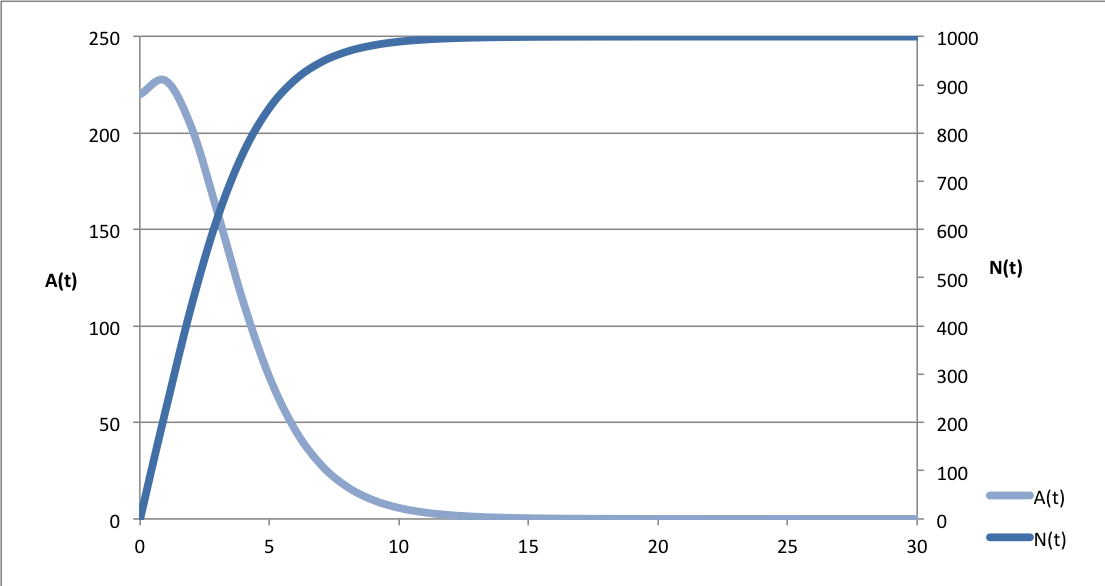
The time scale can be adjusting by observing that the volume of adoption during the first period is $pm$ , therefore choosing annual figures will result in a time scale in years.

Typical values of the coefficients for consumer goods in western markets are p= 0.016 and q = 0.325. The following chart shows adopters and sales for a market size of 1,000.

p = 0.016, q=0.325, m=1,000. 48% of the market at the inflexion point.

There are a number of interesting observations. The coefficient of innovation must be nonzero for the process to work.There is an inflexion point where the curve changes from convex to concave. This coincides with the peak adoption and for the typical values of p and q it occurs at about 48% of market saturation. Moore (1991) argues that adopters are normally distributed, with innovators representing the segment between two and three standard deviations, or about 2.5% of the market, and places a chasm between one and two standard deviations. That point represents about 16% of the market size and corresponds to the inflexion point in the normal distribution.

p=0.22, q=0.325, m=1,000. 16% of the market at the inflexion point

The situation described by Moore would correspond to a coefficient of innovation of 0.22 which is very aggressive and atypical.

The model is based on a number of assumptions

The market potential and composition remains constant over time
The market is geographically homogeneous. Participants share similar values and culture
The diffusion of one innovation is independent of any other innovation
Adoption is modelled as a step function with instant transition
Marketing activities remain constant and do not affect the diffusion process
There are no supply restrictions
Adoption is an individual decision
The adopter adopts a single product

The timing of the peak adoption which is also the inflexion point is sensitive to the coefficient of innovation $p$ .

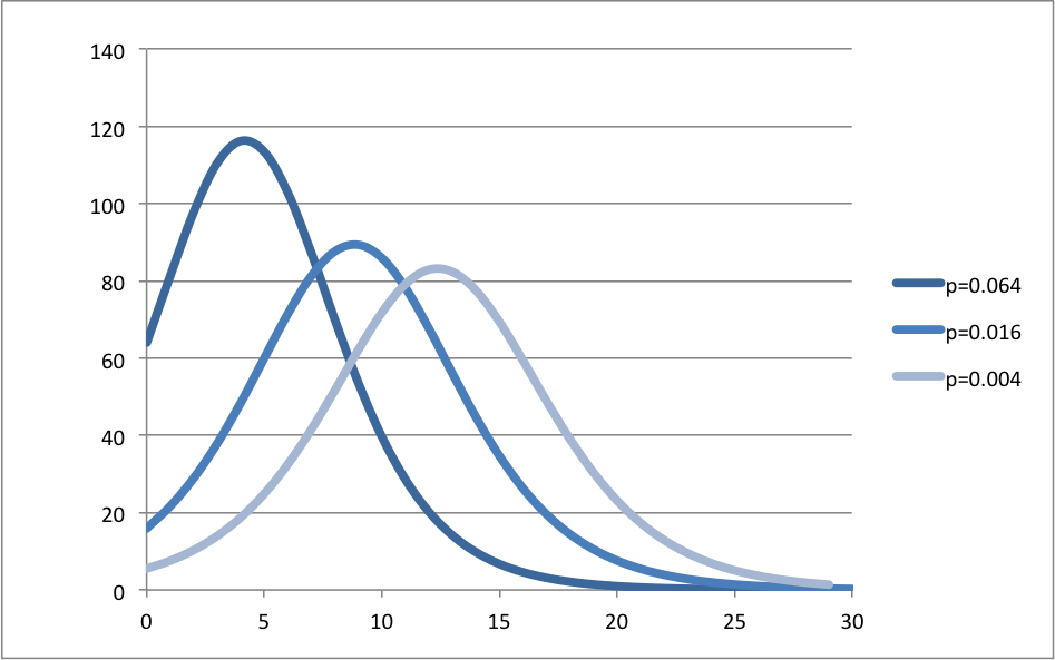
Effect of the innovation parameter

The coefficient of innovation 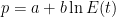$p = a + b\ln E(t)$ depends on three parameters related to marketing and promotion; advertising can modifying the behaviour of innovators and increase early adoption.

Determination of the model parameters using sampling data

The model requires knowledge of the market size and the two coefficients. This information can be estimated from sample data using regression by least squares.

The equation for the number of adoptions can be re-aranged as follows

$A(t) = -\displaystyle\frac{q}{m}N^2(t)+(p+q)N(t)+pm$

This is a second degree polynomial in N(t). For simplicity we can use the following variable substitution where a, b and c depend exclusively on the parameters p, q and m.

$a = -\displaystyle\frac {q} {m}$
$b = (q-p)$
$c = pm$

The sum of squares can be constructed for minimization

$M = \sum\limits_{k=1}^n (A_k-(aN_k^2+bN_k+c))^2$

The minimum value of M is determined by the parameters a,b and c which can be calculated by resolving the system of partial derivatives of M and equating to 0

$\displaystyle\frac{\partial M}{\partial a} = 2 \sum_{k=1}^n(-A_k(t)N_k^2 (t)+ aN_k^4 (t)+ bN_k^3 (t)+cN_k^2 (t)) = 0$
$\displaystyle\frac{\partial M}{\partial b} = 2 \sum_{k=1}^n(-A_k(t)N_k(t) + aN_k^3(t) + bN_k^2(t) +cN_k(t)) = 0$
$\displaystyle\frac{\partial M}{\partial c} = 2 \sum_{k=1}^n(-A_k(t) + aN_k^2(t) + bN_k(t)+c) = 0$

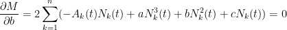
A check of second order derivatives assures that the solution is a minimum

$\displaystyle\frac{\partial^2 M}{\partial a^2} = 2\sum_{k=1}^nN_k^4 (t) > 0$
$\displaystyle\frac{\partial^2 M}{\partial b^2} = 2\sum_{k=1}^nN_k^2 (t) > 0$
$\displaystyle\frac{\partial^2 M}{\partial c^2} = 2n > 0$

The system of equations can written in matrix form and solved using a spreadsheet, provided that the matrix is non-singular.

$\left[ \begin{array}{ccc} \sum\limits_{k=1}^nN_k^4(t) & \sum\limits_{k=1}^nN_k^3(t) & \sum\limits_{k=1}^nN_k^2(t) \\ \sum\limits_{k=1}^nN_k^3(t) & \sum\limits_{k=1}^nN_k^2(t)& \sum\limits_{k=1}^nN_k(t) \\ \sum\limits_{k=1}^nN_k^2(t) & \sum\limits_{k=1}^nN_k(t) & n \end{array} \right] \times \left[ \begin{array}{c} a \\ b \\ c \end{array} \right] = \left[ \begin{array}{c} \sum\limits_{k=1}^nA_k(t)N_k^2(t) \\ \sum\limits_{k=1}^nA_k(t)N_k(t) \\ \sum\limits_{k=1}^nA_k(t) \end{array} \right]$

The coefficient of determination $r^2$ is given by:

$r^2 = 1-\displaystyle\frac{\sum\limits_{k-1}^n \left( A_k(t)-\left( p+q\displaystyle\frac{N_k(t)}{m})(m-N_k(t)\right) \right) ^2}{\sum\limits_{k=1}^n \left(A_k(t)-\displaystyle\frac{\sum\limits_{k=1}^n ( p+q \displaystyle\frac{N_k(t)}{m})(m-N_k(t))}{n}\right)^2}$

References

Bass, F (1969) “A new Product Growth for Model Consumer Durables”
Moore, G (1991) “Crossing the Chasm”
Rogers, E (1972) “Diffusion of Innovations”

Rob Jeges

Management Science and Philosophy

Diffusion of innovation

Abstract

Introduction

The Bass model

Determination of the model parameters using sampling data

References