Introduction

There are many situations where a service is provided by a limited number of agents; the total time to complete a transaction equals the period of waiting time plus the service time. Queuing theory has its roots in telephony where a limited number of connections is available to customers to make a call. If the connections are busy then the customer has to wait until a line becomes available. This model can be extended to services such as contact centres, support teams, checking points, etc. This article develops the theory and provides some practical advice for the application of queuing models using spreadsheets.

There are many possible variants, such as priority of service, restrictions on the queue,etc. We shall deal with the most common situation as shown in the diagram.

There are a number of questions that are important for the design of optimal service management systems:

$\Pr(T_w > 0)$ Probability that a customer has to wait
$E(T_w)$ Average waiting time
$\Pr(T_w \le \tau)$ Probability of being served within a target time

To answer these questions we make the following assumptions:

The system can accommodate an infinite number of customers
The customer does not leave the system until served
The arrival rate follows a Poisson process, meaning that the time between customer arrivals is random with mean time $\lambda$
The Service time of each customer is exponentially distributed with mean time $1/\mu$
The number of servers is $s$

Derivation

Let $\Pr(k)$ = probability that there are $k$ customers in the system. The system is in equilibrium when the probability of a customer entering the system is equal to the probability of a customer leaving the system.

We can analyse this situation by considering the transition between two adjacent states.

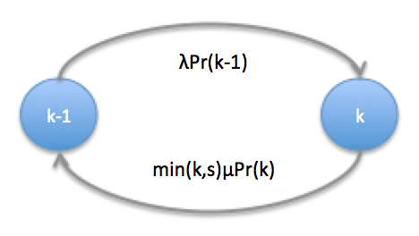
The assumption of exponential service times implies that when there are $k \le s$ customers being served the rate at which service completions occur is $k\mu$ and when all servers are busy only the customers that are being served can leave at a rate of $s\mu$ .

These equations can be combined recursively to obtain:

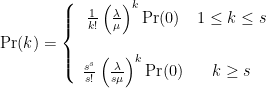
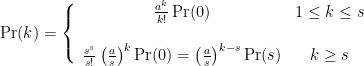
$\Pr(k) = \left\{ \begin{array}{cc} \frac{1}{k!}\left(\frac{\lambda}{\mu}\right)^k\Pr(0) & 1 \le k \le s \\ \; & \; \\ \frac{s^s}{s!} \left( \frac{\lambda}{s\mu} \right) ^k \Pr(0) & k \ge s \end{array} \right.$

We define following useful quantities:

Traffic intensity: $a = \lambda/\mu$
Server utilisation: $\rho = a/s$

To determine $\Pr(0)$ we use the boundary condition $\sum_{j=1}^\infty \Pr(j)=1$

$Pr(0) = \left[ \sum\limits_{j=0}^{s-1}\frac{a^j}{j!} + \frac{s^s}{s!}\sum\limits_{j=s}^ \infty \left(\frac{a}{s} \right)^j \right]^{-1}$

When $\rho <1$ the system is in equilibrium and the infinite sum on the right term converges.

$\Pr(0) = \left[\sum\limits_{j=0}^{s-1}\frac{a^j}{j!} + \displaystyle\frac{a^s}{(s-1)!(s-a)}\right]^{-1}$

The probability distribution for the number of customers in the system is:

$\Pr(k) = \left\{ \begin{array}{cc} \frac{a^k}{k!} \Pr(0) & 1 \le k \le s \\ \; & \; \\ \frac{s^s}{s!}\left(\frac{a}{s}\right)^k \Pr(0)= \left( \frac{a}{s} \right)^{k-s} \Pr(s) & k \ge s \end{array} \right.$

Probability that a customer has to wait

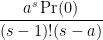
Customers that arrive when all the servers are busy must wait in the queue, and the probability is given by:

${\Pr(T_w > 0)} =$	$\sum\limits_{j=s}^\infty \Pr(j)$
	$\sum\limits_{j=s}^\infty \left( \frac{a}{s} \right)^{j-s} \Pr(s)$
	$\displaystyle\frac{s\Pr(s)}{s-a}$
	$\displaystyle\frac{a^s\Pr(0)}{(s-1)!(s-a)}$
	$\frac{\displaystyle\frac{a^s}{(s-1)!(s-a)}}{\sum\limits_{j=0}^{s-1}\frac{a^j}{j!}+\displaystyle\frac{a^s}{(s-1)!(s-a)}}$

Multiplying the numerator and denominator by $e^{-a}(1-\rho)$ we get the Erlang-C formula:

$E_c(s,a) = \displaystyle\frac{e^{-a}a^s/s!}{e^{-a}a^s/s!+(1-\rho)e^{-a}\sum\limits_{j=0}^{s-1}\frac{a^j}{j!}}$

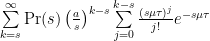
We can re-write this function using the Poisson distribution:

$E_c(s,a) = \displaystyle\frac{P\!oisson_{pmf}(s,a)}{P\!oisson_{pmf}(s,a)+(1-\rho)P\!oisson_{cum}(s-1,a)}$

Where $P\!oisson_{pmf}$ is the Poisson distribution probability mass function, and $P\!oisson_{cum}$ is the Poisson distribution cumulative function. These formulas are available in popular spreadsheet software.

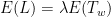
Average waiting time

To calculate the average waiting time $E(T_w)$ we use Little’s formula $E(L) = \lambda E(T_w)$

The expected number of customers in the queue is:

$E(L) = \sum\limits_{k=s+1}^\infty(k-s)\Pr(k) = \displaystyle\frac{as\Pr(s)}{(s-a)^2}$

$E(T_w) = \displaystyle\frac{1}{\lambda}\displaystyle\frac{as\Pr(s)}{(s-a)^2} = \displaystyle\frac{\Pr(T_w>0)}{s(1-\rho)\mu}$

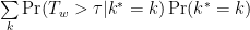
Service Level

We calculate $\Pr(T_w > \tau)$ = probability that a customer has to wait longer than a target time $\tau$ by considering a saturated system where all servers are busy during an interval of time $\tau$ . The number of customers leaving the system during the time $\tau$ follows a Poisson distribution with mean $s\mu \tau$ . Let $k^*$ = the number of customers in the system immediately before an arrival, then:

$\Pr(T_w > \tau | k^* = k) = \sum\limits_{j=0}^{k-s}\displaystyle\frac{(s \mu \tau)^j}{j!}e^{-s\mu \tau}$

From the theorem of total probability and the PASTA property of Poisson distributions:

$\Pr(T_w > \tau) =$	$\sum \limits_k\Pr(T_w > \tau \| k^* = k)\Pr(k^*= k)$
	$\sum \limits_{k=s}^\infty \Pr(s) \left(\frac{a}{s}\right)^{k-s} \sum\limits_{j=0}^{k-s}\frac{(s\mu\tau)^j}{j!}e^ {-s\mu\tau}$
	$\Pr(s) e^{-s\mu\tau} \sum \limits_{j=0}^\infty\frac{(s\mu\tau)^j}{j!} \sum\limits_{k=s+j}^\infty \left(\frac{a}{s}\right)^{k-s}$
	$\Pr(s) e^{-s\mu\tau} \sum\limits_{j=0}^\infty \frac{(s\mu\tau)^j}{j!} \left(\frac{a}{s}\right)^j \frac{s}{s-a}$
	$\frac{s\Pr(s)}{s-a}e^{-s\mu\tau} \sum\limits_{j=0}^\infty\frac{(a\mu\tau)^j}{j!}$
	$\Pr(T_w>0)e^{-(s-a)\mu\tau}$

The probability that a customer will be served within a target time $\tau$ is given by:

$\Pr(T_w \le \tau) = 1 - \Pr(T_w > \tau)$

Applications

A practical question is the number of servers required to provide a given service level. To answer this question a model is build with $s, \lambda$ , and $\mu$ as parameters and $E(T_w)$ and $\rho$ as outputs. By changing the number of servers one can monitor the service level and the server utilisation to determine the optimal numbers.

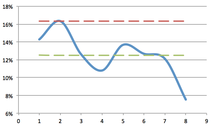
Recalling that customer arrivals follow a Poisson process with mean arrival rate $\lambda$ it is important to note that customer arrivals are not evenly distributes throughout the day. The following picture shows a typical arrival pattern over 8 hours.

Calculating the number of servers to meet an average customer arrival rate $\lambda$ over the entire range will result in periods where the service level is not achieved. To alleviate this situation only the peak period is used to determine $\lambda$ . This results in periods of under utilisation $(\rho <<1 )$ .

The mean service time is also determined over the entire range of services. To model the provision of services with different durations by shared servers, each service can be modelled using the total number of servers. The number of servers can then be adjusted to provide the desired service provided that the total utilisation is not exceeded so the system operates in a stable state:

$\sum \rho \le 1$ .

Conclusion

We have discussed the M/M/c or Blocked customers delayed model, and is the departure point for the analysis of more complex situations such as priority queues and abandonment. All these models can be analysed using similar techniques to those described in this article.

The system parameters are:

Customer arrival rate $\lambda$
Mean service time $1/\mu$
Number of servers $s$

The performance of the system is characterised by:

The probability that a customer has to wait $\Pr(T_w>0)$
The mean waiting time $E(T_w)$
The probability that a customer will be served within a target time $\Pr(T_w \le \tau)$
The server utilisation $\rho$

References

Cooper, R. (1981) “Introduction to Queuing Theory”
Kleinrock, L. (1975) “Queuing Theory”

Rob Jeges

Management Science and Philosophy

Application of Queuing Theory to Capacity Planning